📺 Today’s recommended deep-dive video: https://www.youtube.com/watch?v=xslYf8XHa54

Beyond Clean Data: Generative Modeling via Self-Consistent Transport under Black-Box Corruption

Generative models are powerhouse tools for science, yet they typically rely on a luxury scientists often lack: large pools of perfectly clean data. Zichen Han introduces a paradigm shift by leveraging measure transport to learn clean distributions directly from corrupted observations and black-box simulators.

Core Question: How can we train generative models for clean data when we only have access to corrupted measurements and a forward simulator?

Highlights

• Adapting pre-trained models via modified initial distributions for linear inverse problems.
• Improving Sequential Monte Carlo (SMC) inference scaling through variance-controlled drift.
• The “Self-Consistent Stochastic Interpolant” framework for training without clean data.
• Applications across image restoration, JPEG decompression, and cosmological spectral analysis.

⏱️ Reading time: approx. 8 minutes · Saves you about 60 minutes vs. watching.

Want to take notes while watching? Click the image below and let AI Notebook capture the key points for you 👇

The Adaptation Problem in Measure Transport

Beyond Standard Clean-Data Prior Training

Generative modeling isn’t just about recreating the training set; it’s about steering it toward specific, high-value outcomes.

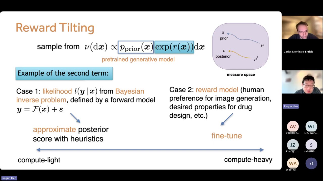
Traditional methods modify reverse dynamics with heuristics, but these lack theoretical guarantees and often introduce uncontrollable bias errors during sampling. These approximations work for simple tasks, but they fail to scale when high precision or complex reward functions are required for scientific validity.

Zichen Han presents a new way to fix this: one involves starting the diffusion process from a non-Gaussian log-concave distribution for linear problems, while another utilizes variance-controlled drift. By optimizing the proposal drift within a simple linear subspace of basis functions—specifically reward gradients and prior scores—researchers can achieve true inference-time scaling. This means that increasing the number of particles actually translates to observable accuracy gains, rather than hitting a variance-induced performance ceiling as seen in basic guidance methods.

💡 Digging Deeper

Q: Why modify the initial distribution rather than the dynamics?
A: In linear inverse problems, it is mathematically more robust to change the “starting point” from a standard Gaussian to a specific log-concave distribution that inherently contains posterior information.

Q: What is the primary limitation of Sequential Monte Carlo (SMC) in diffusion?
A: Particle methods often suffer from extreme weight variance, causing the effective sample size to collapse before reaching the target distribution.

Q: How does drift control solve this?
A: It solves a Poisson equation to find an optimal control that minimizes weight variance, effectively “pushing” particles toward the target more efficiently.

Learning from Corruption

The Challenge of Indirect Scientific Observations

In fields like cosmology or cryo-EM, “clean data” is essentially a myth; we only possess noisy measurements and a simulator representing the physics of the corruption.

The goal is to solve the distribution-level equation $Kpi = mu$ for the clean distribution $pi$.

The proposed solution is the “Self-Consistent Stochastic Interpolant,” a bi-level iteration scheme that requires only a black-box simulator. In the outer loop, a fixed-point iteration guesses the clean distribution, while the inner loop optimizes a transport map between this guess and its simulated corruption. This cycle continues until the model achieves self-consistency, effectively learning the clean data prior without ever seeing a single uncorrupted sample. This is particularly powerful because it doesn’t require the likelihood function to be differentiable or even explicitly known.

Practical Performance and Theoretical Rigor

Scaling to High-Dimensional Scientific Data

Theoretical rigor supports this framework, demonstrating linear convergence in Gaussian settings even when the signal-to-noise ratio is extremely low.

Experiments on CelebA show that even highly non-linear, non-differentiable corruptions like JPEG compression can be reversed using this black-box approach. The model learns to de-compress and restore features by observing only low-quality, artifact-heavy images and knowing the compression algorithm’s parameters.

When compared to standard posterior sampling methods like DPS (Denoising Diffusion Posterior Sampling), this self-consistent approach often yields higher restoration quality. Because it leverages the entire dataset distributionally rather than solving inverse problems point-by-point, it captures structural nuances that individual restoration attempts miss. In cosmology applications, this translates to significantly better spectral resolution from low-quality signals, proving that joint distribution-level modeling is superior to sample-level optimization.

💡 Digging Deeper

Q: How does this differ from the classical Expectation-Maximization (EM) algorithm?
A: EM requires an explicit likelihood and reliable posterior sampling; this method uses a black-box simulator and converges faster by avoiding the E-step’s sampling bottleneck.

Q: Is the bi-level optimization computationally expensive?
A: While it requires an outer loop, the inner loop iterations can be kept small—often just 10 to 20 steps—making the total overhead roughly 10x that of standard training.

Q: Does the ODE or SDE variant converge faster?
A: Theoretical analysis and empirical results suggest that the ODE case (zero diffusion) typically achieves the fastest convergence in the fixed-point iteration.

Key Takeaways

Measure transport provides a flexible mathematical language for both generating and adapting data distributions. By treating generative modeling as a dynamical system, we can steer outputs through reward tilting or posterior sampling with much higher precision than traditional heuristic guidance allows. The introduction of drift control specifically enables “inference-time scaling,” allowing computational power to directly translate into better samples.

The shift from sample-level inverse solvers to distribution-level “Self-Consistent Transport” marks a major milestone for scientific machine learning. It allows researchers to train high-quality generative priors in domains where clean training data is unavailable, such as medical imaging or astronomy. As long as a simulator for the corruption exists, the clean truth can be recovered through iterative consistency.

Ultimately, these tools move generative AI from the realm of “interpolation of clean images” into a robust framework for scientific discovery. By leveraging the joint information across entire corrupted datasets, we can reconstruct the underlying reality of physical systems with a level of detail that individual measurements cannot provide.

Q&A

Q1: What happens if the forward simulator is not perfectly accurate?
A1: The current framework assumes a perfect simulator. If mis-specification exists, the model may converge to a biased prior. Future work involves integrating uncertainty quantification for forward model parameters into the bi-level loop.

Q2: How much data is required for self-consistent training?
A2: Surprisingly, standard datasets like CIFAR-10 are sufficient. The gap between clean-data training requirements and corrupted-data training is modest, usually within the same order of magnitude.

Q3: Can this method handle non-differentiable corruption like JPEG?
A3: Yes. Because the method only requires black-box access to the simulator (generating $Y$ from $X$), it does not need to backpropagate through the corruption process itself.

Q4: How does this work for conditional models, such as protein generation?
A4: For conditional models, one can optimize the conditional embeddings themselves. This shifts the prior toward the desired target distribution while keeping the protein structures physically plausible.

Q5: Why is the “fixed-point” iteration necessary?
A5: Since we lack clean samples ($X$), we must use our current best guess of the clean distribution to define the transport map, then refine that guess based on how well the simulated corruption matches the actual observations.

Q6: Does this framework support both ODE and SDE dynamics?
A6: Yes, it is unified under stochastic interpolants. While SDEs offer more stochasticity, the ODE variants often show faster convergence in the self-consistency iterations.

Q7: Can this be used for real-time inference?
A7: The inference-time scaling work is specifically designed to make real-time sampling more accurate by efficiently using available compute to reduce particle variance.