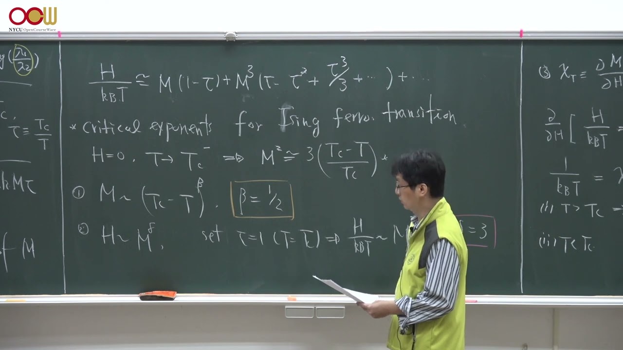
📺 Today’s recommended deep-dive video: https://www.youtube.com/watch?v=8y5bQtzE8Vg

Beyond the Infinite Range: Mean Field Theory and the Birth of Landau’s Universal Framework

Transitioning from toy models to realistic lattices requires a shift in how we view local interactions. By replacing complex neighbor interactions with a single “effective field,” we unlock a universal language that allows us to compare magnets, fluids, and superconductors through the same mathematical lens.

Core Question: How does Mean Field Theory bridge the gap between specific physical systems and Landau’s universal theory of phase transitions?

Highlights

• The Weiss Mean Field approximates neighbor interactions as a singular effective magnetic field.
• Derivation of universal critical exponents ($beta=1/2, delta=3, gamma=1$) reveals MFT’s strengths and its failure to account for dimensionality.
• Order parameters serve as the defining metric for distinguishing ordered states from disordered ones across various physical systems.
• Landau Theory postulates that free energy can be expanded as a power series of the order parameter near the critical point.

⏱️ Reading time: approx. 6 minutes · Saves you about 35 minutes vs. watching.

Want to take notes while watching? Click the image below and let AI Notebook capture the key points for you 👇

The Mechanics of Mean Field Theory

The Weiss Effective Field

In a realistic Ising model, every spin is influenced by its neighbors. Instead of tracking every individual interaction, Weiss Mean Field Theory simplifies the local environment by assuming each spin experiences an “effective field.” This field combines the external magnetic force with the average influence of all surrounding neighbors, effectively “averaging out” the complexities of the lattice.

The self-consistency of this model arises because the magnetization influencing the neighbors is the same magnetization we seek to calculate for the entire system.

By summing the couplings across $2D$ neighbors (where $D$ is dimensionality), we arrive at a transcendental equation: $M = tanh(H_{eff}/k_BT)$. Solving this requires finding the intersection between a linear slope and the hyperbolic tangent curve. Below a critical temperature $T_C$, the system exhibits spontaneous magnetization, even when the external field is zero. This marks the transition from a disordered paramagnetic state to an ordered ferromagnetic state, driven purely by internal feedback where every site affects every other site.

💡 Digging Deeper

Q: Why does the Mean Field Theory neglect fluctuations?
A: MFT assumes that each spin only “sees” the average magnetization of its neighbors. It ignores the local deviations or “noise” from that average, which actually becomes very significant as the system nears the critical temperature.

Q: How does dimensionality ($D$) enter the equation?
A: In MFT, dimensionality only appears as a multiplier for the number of nearest neighbors (e.g., $2D$ for a cubic lattice). However, it does not change the resulting critical exponents, which is a known inaccuracy of the theory.

Extracting the Universal Exponents

Breaking Down the Power Laws

Near the critical point, we can Taylor expand the free energy because the magnetization $M$ and the external field $H$ are infinitesimal. This expansion reveals the “equation of state,” which links temperature, field, and order. From here, we derive the critical exponents: $beta = 1/2$ for spontaneous magnetization, $delta = 3$ for the field dependence at $T_C$, and $gamma = 1$ for the divergence of isothermal susceptibility as the system approaches criticality.

Strikingly, these exponents remain constant regardless of whether the lattice is one-dimensional or three-dimensional, highlighting a major limitation of basic Mean Field Theory.

While MFT provides a robust starting point, it neglects the spatial fluctuations that become dominant near $T_C$. In reality, the dimensionality of the lattice significantly alters the behavior of real-world materials—for instance, a 2D Ising model has different exponents than a 3D one. To fix this, we must look toward Landau’s more generalized approach, which focuses on symmetry and order parameters rather than specific lattice geometry.

Landau Theory and the Order Parameter

From Magnetism to Superfluidity

Lev Landau’s genius lay in his realization that all phase transitions share a common DNA. He introduced the “order parameter”—a scalar or vector that is zero in the disordered phase and non-zero in the ordered phase. This allows us to map the Ising model directly onto liquid-gas transitions, where the difference in density serves as the order parameter.

The complexity of the order parameter varies by system: it is a simple scalar for Ising models, a vector for Heisenberg magnets, and a complex wave function for superconductors. In the case of liquid helium-3, the order parameter has a staggering 18 components, accounting for both spin and orbital symmetries. Regardless of the physical nature of these components, Landau proposed that the free energy could always be expanded as a power series of these parameters near the transition point.

This universality means that a fluid near its critical point and a magnet near its Curie temperature are governed by the exact same mathematical symmetries.

Key Takeaways

Mean Field Theory serves as a powerful, albeit crude, approximation for understanding how local spin interactions lead to global ordering. By replacing the sum of neighboring spins with an effective “Weiss field,” we can derive a self-consistent equation for magnetization. This method successfully predicts the existence of a phase transition and provides a set of universal critical exponents ($beta, delta, gamma$).

However, the theory’s primary weakness is its indifference to dimensionality. Because it ignores the spatial fluctuations that occur near the critical temperature, it predicts the same behavior for a 1D chain as it does for a 3D crystal. This discrepancy led to the development of Landau Theory, which abstracts the physics of the transition into a “free energy functional” based on the symmetry of an order parameter.

Ultimately, Landau’s framework reveals that phase transitions are not just properties of specific materials, but universal phenomena. Whether we are looking at the spontaneous magnetization of iron or the pairing of electrons in a superconductor, the mathematical structure of the transition remains remarkably consistent. This provides the foundation for modern statistical mechanics and the study of topological phases of matter.

Q&A

Q1: What is the “spontaneous magnetization” mentioned in the lecture?
A1: It is the magnetization that remains in a material even after an external magnetic field is removed, occurring only when the temperature is below the critical point ($T_C$).

Q2: How does the Ising model relate to a liquid-gas transition?
A2: They are mathematically equivalent; the “up” and “down” spins of the Ising model correspond to the presence or absence of particles (density) in a fluid.

Q3: What is the Kosterlitz-Thouless (KT) transition?
A3: It is a special phase transition in 2D systems (like thin-film superconductors) driven by the pairing and unpairing of topological defects called vortices, rather than standard symmetry breaking.

Q4: Why are critical exponents like $beta=1/2$ considered “universal”?
A4: They are called universal because they depend only on the symmetry of the order parameter and the dimensionality of the system, not on the specific details of the atomic interactions.

Q5: What happens to the order parameter at temperatures above $T_C$?
A5: Above $T_C$, the system is in a disordered state (like a paramagnet or a gas), and the order parameter vanishes to zero.

Q6: What is a “self-consistent equation” in this context?
A6: It is an equation where the variable you are trying to solve for (Magnetization, $M$) appears on both sides of the equals sign, requiring an iterative or graphical solution.

Q7: What is the significance of the 2016 Nobel Prize mentioned?
A7: It was awarded to Kosterlitz, Thouless, and Haldane for their work on topological phases and transitions, which expanded our understanding of matter beyond Landau’s original symmetry-breaking framework.