📺 Today’s recommended deep-dive video: https://www.youtube.com/watch?v=c7sT6RlCbTo

Wave Function Flows: Inference Through Quantum Interference

Generative AI and quantum physics are often viewed as separate worlds, but recent research reveals they share a deep mathematical foundation. By mapping continuous flow models to the Schrödinger equation, researchers have unlocked a way to perform inference through quantum interference, turning diffusion models into “quantum mechanics in disguise.”

Core Question: Can we efficiently simulate continuous flow models on quantum computers to gain more powerful access to learned distributions?

Highlights

• Continuous flow models (diffusion, flow matching) map naturally to the Schrödinger equation via a “Wave Function Flow” transformation.
• Quantum computers provide a quadratic speedup for downstream tasks like mean estimation through coherent encoding (Q-sampling).
• The “Continuity Hamiltonian” bridges the gap between machine learning velocity fields and the kinetic/potential energy terms found in physical laws.
• This mapping creates a “Rosetta Stone” for understanding the complexity and representational limits of generative models using quantum complexity theory.

⏱️ Reading time: approx. 8 minutes · Saves you about 45 minutes vs. watching.

Want to take notes while watching? Click the image below and let AI Notebook capture the key points for you 👇

Quantum Mechanics as Probability Theory

The Shift to the 2-Norm

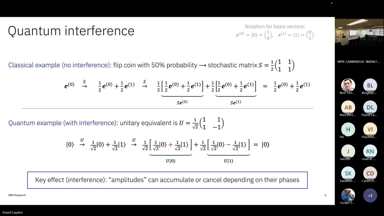
Quantum mechanics is essentially probability theory with two distinct tweaks: the use of complex numbers and the adoption of the L2 norm. In classical probability, we deal with non-negative vectors that sum to one, representing the mass of specific outcomes. Quantum mechanics replaces these with wave functions where the probability density is determined by the absolute value squared of a complex amplitude.

This transition from real numbers to complex amplitudes introduces the phenomenon of interference, where paths can cancel each other out or reinforce one another. Consider a coin flip: while two classical flips always lead to a uniform distribution, two quantum “flips” can interfere destructively, returning the system to its original state with absolute certainty. This “quantumness” allows for computation that classical logic simply cannot replicate.

Interference and the Dynamite Puzzle

The power of quantum states is best illustrated by the Elitzur-Vaidman bomb tester thought experiment. Imagine a bomb so sensitive that a single photon triggers it, but some bombs are duds with no triggers. Classically, you cannot identify a working bomb without risk, but quantum interference allows a photon to “sense” the trigger without interacting with it. By splitting a photon’s path and looking for specific interference patterns, you can certify a bomb is functional even if the photon never touched the fuse.

💡 Digging Deeper

Q: Why are complex numbers used instead of just negative probabilities?
A: Complex numbers provide a phase that allows for rotation and preservation of the L2 norm during evolution, which is required for unitary (reversible) dynamics.

Q: Is a Q-sample just a regular sample?
A: No, a Q-sample is a coherent quantum state that, when measured, yields a sample, but before measurement, it can be manipulated using quantum gates.

The Quantum Computing Landscape

Hardware and the Noise Barrier

Quantum computers are not universal panaceas; they are specialized tools that excel at simulating the Schrödinger equation while struggling with large data inputs. The main barrier to modern quantum utility remains hardware noise and the difficulty of loading massive classical datasets into a quantum state. While algorithms like the HHL linear system solver offer theoretical exponential speedups, they often become bottlenecked by the time required to simply define the input vector.

To overcome these limitations, researchers focus on “native” tasks where the quantum system naturally reflects the problem structure. Simulating physical dynamics is the primary use case, as it avoids the messy process of calculating high-dimensional matrices. Instead, the computer uses a sequence of discrete logic gates to approximate continuous evolution through techniques like Trotterization or Euler-style time-stepping.

Native Simulation

Richard Feynman famously proposed that to simulate nature, one must build a machine that is itself quantum mechanical. Modern quantum computers implement this by toggling between different components of a Hamiltonian—such as kinetic and potential energy—to evolve a state forward in time. Because these machines natively understand the Schrödinger equation, they can solve certain differential equations far more efficiently than classical silicon chips.

💡 Digging Deeper

Q: Can quantum computers solve any NP-hard problem?
A: Generally, no; we expect them to be good at specific problems like factoring or simulating physics, but not for finding global minima in arbitrary landscapes.

Q: What is a logic gate in a quantum context?
A: It is a calibrated unitary operation, such as a rotation, that manipulates the quantum state’s amplitudes without collapsing them.

Wave Function Flows: The Mapping

From Continuity to Schrödinger

The core of this discovery is the Wave Function Flow, a direct mathematical bridge between generative ODEs and quantum evolution. By taking the square root of the probability density, researchers found that the time derivative of a learned distribution follows a specific first-order differential equation. This equation perfectly matches the Schrödinger form, provided we define a specialized linear operator known as the Continuity Hamiltonian.

This mapping means that every diffusion model or flow-matching model is effectively a recipe for a quantum system. You can take the velocity field learned on a GPU and “re-run” it on a quantum processor. Instead of moving points through a vector field, the quantum computer evolves the entire probability wave function simultaneously through unitary gates.

The Continuity Hamiltonian

When the velocity field is conservative—meaning it is the gradient of a scalar function—the resulting Hamiltonian splits into two familiar physical components. The first term mirrors kinetic energy through a Laplacian operator, while the second acts as potential energy derived from the learned velocity field. This structural identity suggests that flow models are not just analogies, but physical systems we can simulate.

💡 Digging Deeper

Q: Does this require new training methods for AI?
A: No, you can use existing velocity fields from pre-trained diffusion models and map them directly to the quantum Hamiltonian.

Q: What is a “conservative” velocity field?
A: It is a field where the flow depends only on the potential difference between points, similar to gravity or the score function in diffusion.

The Future of Quantum Inference

Inference Through Interference

Quantum access offers a quadratically faster route to estimating means and expectations through a technique known as amplitude estimation or coherent state manipulation. Beyond simple speedups, this framework allows researchers to apply non-local operations like the Discrete Fourier Transform directly to the learned distribution. This capability enables the discovery of hidden structural patterns that would be computationally intractable to extract using standard Monte Carlo sampling methods.

The Rosetta Stone of Complexity

There is also a significant theoretical implication regarding the “Rosetta Stone” effect, which translates complexity bounds between the two fields. If certain distributions are proven to be hard to prepare as quantum states, it implies fundamental limits on the ability of any flow-based model to learn those specific distributions. This connection provides a new lens for understanding the representational capacity of modern AI.

💡 Digging Deeper

Q: Will this make image generation faster?
A: Not necessarily for just getting a single image, but it makes analyzing the statistics of the generated distribution much faster.

Q: Can we use this for discrete data?
A: Discrete diffusion is actually more “natural” for quantum computers since they are discrete-state machines, making it a promising area for future work.

Key Takeaways

The mapping of generative flow models to quantum Schrödinger dynamics represents a fundamental bridge between machine learning and physics. By treating the square root of a probability density as a wave function, we can leverage the unique strengths of quantum computers—specifically their ability to simulate unitary evolution—to probe AI models in ways that were previously impossible. This allows for “Inference through Interference,” where complex amplitudes are manipulated to reveal global properties of a distribution with fewer samples than classical methods.

While current quantum hardware is too noisy to run these simulations at scale, the theoretical groundwork is now set. This “Wave Function Flow” framework not only promises future speedups for scientific AI tasks but also provides a new set of complexity-theoretic tools to analyze why certain distributions are easy or hard for models like Stable Diffusion to learn. As quantum technology matures, our ability to interact with the high-dimensional distributions learned by AI will shift from stochastic sampling to coherent manipulation.

Q&A

Q1: Does this approach require a specific type of quantum computer?
A1: The mapping is general, but it is best suited for “digital” quantum computers capable of universal gate operations, like those being developed by IBM or Microsoft.

Q2: How much faster is the quantum mean estimation?
A2: It provides a quadratic speedup, meaning if you needed 1,000,000 samples classically, you might only need 1,000 “quantum samples” to reach the same error tolerance.

Q3: Is the “Continuity Hamiltonian” found in nature?
A3: No, it is a synthetic Hamiltonian that arises specifically from the math of flow models, though it shares the same kinetic and potential energy structure as natural systems.

Q4: Can this be used to train models faster?
A4: Currently, the work focuses on inference; training remains a classical task because of the difficulty of performing backpropagation on quantum hardware.

Q5: What is the biggest hurdle to running this today?
A5: The “discretization error” and noise; current quantum computers lack the coherence time to run the many steps required to simulate a complex flow accurately.

Q6: How does the “Rosetta Stone” help ML researchers?
A6: It allows them to use 40 years of quantum complexity theory to prove what types of data distributions a diffusion model can or cannot learn.

Q7: Does this apply to Large Language Models (LLMs)?
A7: This specific mapping applies to continuous flow models (like diffusion); mapping the discrete, categorical nature of LLMs to quantum dynamics is a separate, more challenging problem.