📺 Today’s recommended deep-dive video: https://www.youtube.com/watch?v=DlJcoEu1uos

Solving the Impossible: Mastering Rare Events Through Stochastic Optimal Control

Predicting how proteins fold or how chemical catalysts behave requires observing events that happen once in a trillion simulation steps. Standard brute-force methods fail, leaving researchers blind to the critical transitions that define biological and physical life. By recasting these rare transitions as a stochastic optimal control problem, we can finally bridge the gap between femtosecond vibrations and second-long transitions.

Core Question: How can we use stochastic optimal control and the committor function to efficiently sample and model rare transitions between metastable states in complex physical systems?

Highlights

• Rare events occur on time scales exponentially separated from normal vibrations, making brute-force simulation impossible.
• The “Committor Function” is the central object of transition path theory, identifying the probability of reaching a target state.
• Recasting the sampling problem as a Stochastic Optimal Control (SOC) problem solves the “chicken and egg” dilemma of rare event sampling.
• Value Matching (VM) provides a rigorous, off-policy learning framework with first-order optimality guarantees for complex, non-reversible systems.

⏱️ Reading time: approx. 11 minutes · Saves you about 58 minutes vs. watching.

Want to take notes while watching? Click the image below and let AI Notebook capture the key points for you 👇

The Rarity Problem and the Committor

The Hidden Mechanisms of the Physical World

Rare events are the ghosts of the physical world, manifesting in everything from the way a drug molecule binds to a receptor to the sudden phase transition of supercooled water. While most of a system’s life is spent vibrating in a stable “metastable” state, the truly interesting behavior happens during the lightning-fast jumps between these states, which are statistically improbable but functionally essential for life.

These transitions are called “rare” because they occur across massive energy barriers that brute-force molecular dynamics simulations simply cannot cross within reasonable human timeframes.

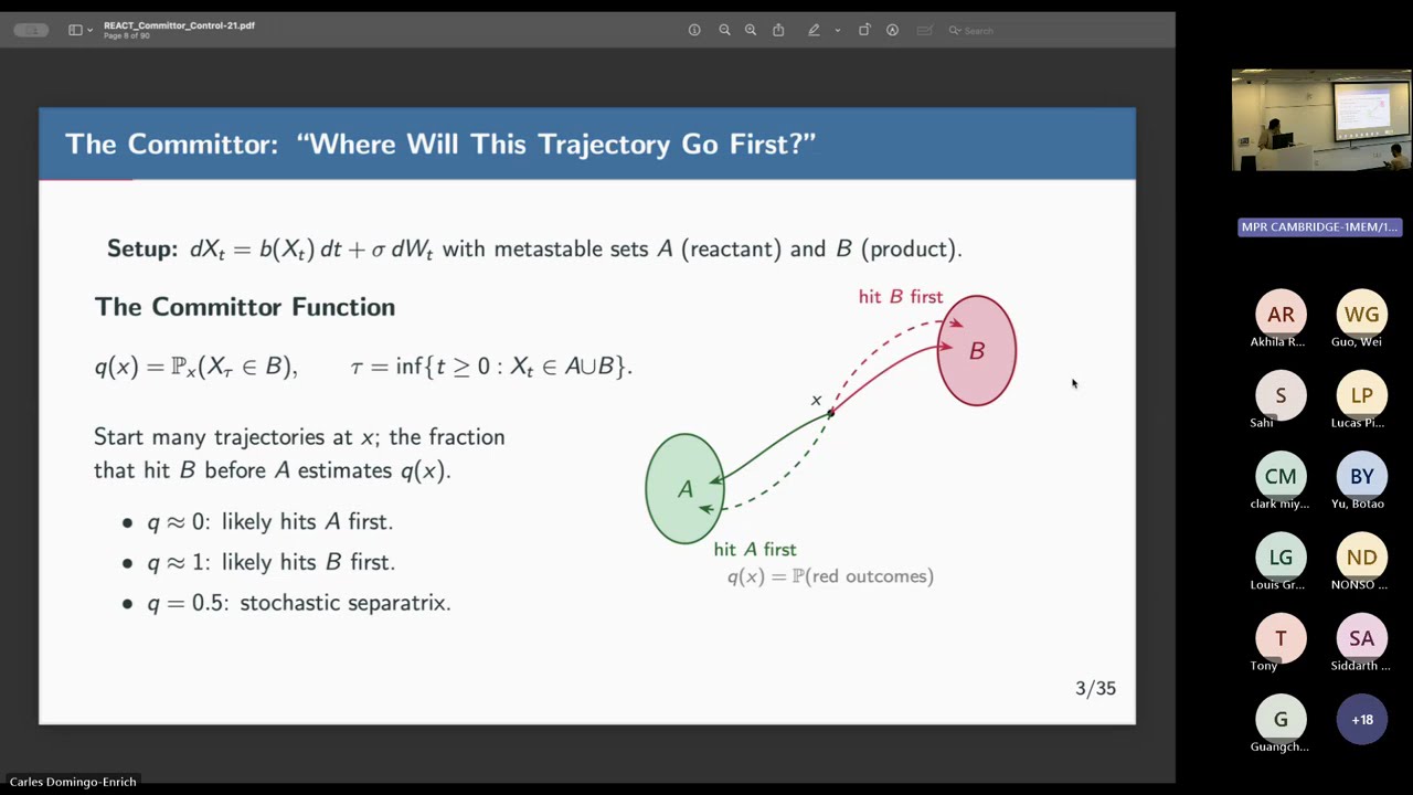
To quantify these jumps, researchers look for the “committor function,” a mathematical value representing the probability that a system starting at a specific point will reach state B before retreating to state A. This function is the holy grail of transition path theory, as it reveals the exact mechanism and rate of the reaction. However, in a high-dimensional space, calculating this probability is like trying to map a dark forest by only looking at the few trees you happen to bump into.

💡 Digging Deeper

Q: Why exactly is brute force simulation impossible?
A: In molecular dynamics, we simulate steps in femtoseconds ($10^{-15}$s). Rare events happen in microseconds to seconds. You would need $10^{15}$ steps just to see one transition, which is computationally unreachable even for supercomputers.

Q: What does it mean for a state to be “metastable”?
A: It is a local minimum in the energy landscape. The system stays there for a very long time, vibrating, until a lucky thermal fluctuation gives it enough energy to jump the barrier to the next minimum.

Control as the Catalyst

From Passive Observation to Active Steering

The traditional way to learn the committor function involves the Kolmogorov backward equation, a linear partial differential equation that describes how the system evolves. However, for most complex, non-reversible biological systems, solving this equation directly is computationally prohibitive and fails to provide samples in the transition regions where they are most needed.

By applying a logarithmic transformation to the committor, researchers can recast the problem as a Hamilton-Jacobi-Bellman (HJB) equation, effectively turning a sampling problem into a stochastic optimal control (SOC) problem.

In this new framework, we are no longer just watching the system; we are learning a “drift” or a steering force that actively pushes the simulation toward the reactive barrier, ensuring we spend our computational budget exactly where the transition happens. This creates a principle-based feedback loop where a better committor estimate leads to better steering, which in turn provides higher-quality data to further refine the committor. It essentially solves the “chicken and egg” problem: you need the committor to sample the transition, and you need the transition samples to learn the committor.

💡 Digging Deeper

Q: What is the “Doob’s h-transform”?
A: It is a mathematical technique to transform a standard Markov process into one that is conditioned to hit a certain set of states. In this talk, it represents the ideal “drift” that perfectly guides a system from A to B.

Q: How does optimal control reduce the variance of our estimates?
A: By steering the system toward the barrier, we observe transitions much more frequently. This “importance sampling” reduces the uncertainty in our rate calculations compared to waiting for a random jump.

Bridging the Gap with Value Matching

Overcoming Rugged Landscapes and Noise

Even with optimal control, rugged energy landscapes—full of tiny local traps—can snag a simulation, preventing it from ever reaching the desired destination. To solve this, the researchers introduced a “noise rescaling” technique inspired by diffusion models, where they reduce the noise level while adding a score-based correction to the drift.

This allows the system to glide over rough terrain more smoothly without losing the underlying physical statistics that make the simulation meaningful for real-world chemistry.

The standout learning method, “Value Matching” (VM), offers a rigorous way to train these models off-policy, meaning we can use trajectories generated at different noise levels to learn the ground truth. Unlike simpler back-propagation methods that struggle with non-differentiable hitting times, Value Matching provides first-order optimality guarantees, making it a robust choice for everything from simple potential wells to complex, time-dependent non-equilibrium systems. It ensures that if the gradient of the loss is zero, we have truly found the optimal committor.

💡 Digging Deeper

Q: What is the benefit of the ‘Value Matching’ loss over ‘Direct Backpropagation’?
A: Direct Backpropagation (DBP) requires differentiating through the “hitting time,” which is mathematically ill-defined and computationally expensive. Value Matching is off-policy and stays stable even when the simulation takes a long time to hit the boundary.

Q: Can this handle non-reversible systems, like a driven motor?
A: Yes. Unlike classical variational methods that require “detailed balance,” the SOC formulation makes no assumptions about reversibility, allowing it to model systems that are periodically driven or have stationary currents.

Key Takeaways

The study of rare events is moving from passive statistical observation to active, control-based learning. By interpreting the committor function through the lens of stochastic optimal control, researchers can bypass the astronomical time scales of molecular dynamics. The introduction of Value Matching and noise annealing allows for the accurate estimation of reaction rates and transition paths in systems that were previously considered “unsimulatable.”

This framework is particularly powerful because it handles non-equilibrium systems where classical physics assumptions often break down. Whether it is a protein switching its shape or a lithium ion moving through a battery electrolyte, these methods provide a clear mathematical path to understanding the “invisible” transitions that govern the physical world. The transition from linear equations to non-linear control problems marks a significant leap in our ability to engineer and discover new molecular processes.

Q&A

Q1: What is the biggest practical hurdle in applying SOC to rare events?
A: The “chicken and egg” problem. You need a decent initial guess for the committor to start steering the system, but if the energy barrier is too high, you might never see a transition to start learning from. The researchers use “collective variables” (like Euclidean distance) to jump-start this process.

Q2: How does the noise rescaling ($kappa$) parameter work?
A: It is an annealing factor. By setting $kappa < 1$, you effectively lower the noise, which helps the system cross barriers faster. A score-based correction is then added to the drift to ensure the marginal distributions remain physically consistent.

Q3: Can these methods be used for discrete state spaces, like a graph of chemical reactions?
A: Yes. The math translates directly from continuous Langevin dynamics to discrete generators on a graph. The principles of the infinitesimal generator and the committor remain the same.

Q4: Is the committor function limited to just two states, A and B?
A: While the talk focuses on A and B for simplicity, the logic extends to multiple states. The committor evaluates the probability of hitting one specific set of states before any other.

Q5: What is the “Rockafeller” potential mentioned in the experiments?
A: It is a version of the Muller potential but with added sinusoidal waves that create a “rugged” energy landscape. This tests the method’s ability to avoid getting stuck in small local minima during a transition.

Q6: Does this approach require knowing the exact energy landscape ($U(x)$)?
A: Yes, the current formulation uses the gradient of the potential energy. However, since the learning is off-policy, it can potentially be adapted to work with noisy or approximate energy estimates in the future.