📺 Today’s recommended deep-dive video: https://www.youtube.com/watch?v=NAx8kKh5iTM

Modeling Uncertainty: Solving Stochastic Heat Inclusions with Fractional Time

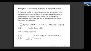
How do we predict the spread of pollutants through porous rocks when the physical environment is full of fractures and unknown variables? This lecture explores a rigorous mathematical framework using fractional calculus and white noise theory to model uncertainty in complex media. Professor Bernt Øksendal details how stochastic distributions and fixed-point theorems can provide solutions for systems where standard differential equations fail.

Core Question: Can we prove the existence of solutions for time-fractional heat inclusions driven by Brownian and Lévy noise, and when do these solutions behave as “mild” square-integrable processes?

Highlights

• Proves that solutions to fractional heat inclusions are fixed points of specific set-valued maps.
• Establishes the existence of solutions using Kakutani’s fixed-point theorem in stochastic distribution spaces.
• Identifies the specific boundaries for “mild” solutions based on fractional order $alpha$ and spatial dimension $d$.
• Applies the theory to environmental scenarios like nitrate pollution in sandy groundwater systems subject to sudden rain-induced jumps.

⏱️ Reading time: approx. 6 minutes · Saves you about 53 minutes vs. watching.

Want to take notes while watching? Click the image below and let AI Notebook capture the key points for you 👇

The Mathematics of Uncertainty

Defining the Inclusion

Differential inclusions are essentially set-valued differential equations where the derivative belongs to a range of possible values rather than a single fixed number.

In practical terms, this allows researchers to model systems where physical parameters like absorption rates aren’t perfectly known, typically resulting in a family of functions as the final solution rather than a unique path, which is particularly useful in complex geotechnical modeling.

When we apply this to fractional heat equations, the inclusion framework accounts for the inherent uncertainty of porous media, where materials like limestone and clay layers create varying degrees of pollutant absorption that a standard deterministic equation might otherwise oversimplify or ignore entirely, leading to a much more robust representation of how substances move through heterogeneous environments like the North Sea’s oil-bearing rocks.

💡 Digging Deeper

Q: Why use a “set-valued” map instead of a standard function?
A: A set-valued map (inclusion) reflects uncertainty. If you don’t know the exact absorption rate of a rock, but know it falls between two values, the inclusion allows the model to account for every possibility within that range.

Q: What does the fractional time derivative represent physically?
A: It models memory and anomalous diffusion. If $alpha < 1$, it represents sub-diffusion (particles move slower/get trapped); if $alpha > 1$, it represents super-diffusion (particles spread faster than normal).

Brownian and Lévy White Noise Frameworks

Beyond Gaussian Noise

The construction of stochastic noise requires a rigorous foundation using the Bochner-Minlos theorem to define probability measures on Schwartz spaces of distributions.

By utilizing the multi-parameter Brownian sheet, we can represent white noise as the derivative of these sheets with respect to both space and time, providing a flexible tool for simulating random microscopic fluctuations in permeability across different dimensions.

While Brownian noise covers Gaussian fluctuations, the inclusion of Lévy white noise allows the model to account for sudden jumps and discontinuities, which are essential for describing fractured systems where particles might be trapped for days before being released suddenly into the flow, a behavior that standard Gaussian models fail to capture effectively in high-dimensional spatial contexts.

💡 Digging Deeper

Q: What is the “White Noise” probability measure?
A: It is often called the Gaussian measure on the space of tempered distributions (S’), providing a mathematical base to treat “noise” as a rigorous random variable.

Q: How does the Lévy sheet differ from standard Brownian motion?
A: A Lévy sheet allows for independent, stationary increments in multi-dimensional time and includes a jump measure (N), which accounts for sudden, large-scale events in the system.

Mild Solutions and Real-World Applications

The Quest for Mildness

A solution is considered “mild” if its expected variance remains finite, meaning it can be represented in a standard square-integrable (L2) form.

Prof. Øksendal demonstrates that mildness depends heavily on the interplay between the fractional order $alpha$ and the space dimension $d$, showing that sub-diffusive models with $alpha < 1$ fail to produce mild solutions regardless of how many dimensions are involved.

In the context of nitrate pollution in sandy groundwater, these mathematical proofs help hydrologists understand why contaminants might spread in ways that defy traditional expectations, particularly when heavy rain or irrigation triggers sudden fractures in the soil, demanding a distribution-based approach to risk assessment that goes beyond simple L2 space calculations and accounts for the extreme variability found in real-world aquifers.

💡 Digging Deeper

Q: When is a solution “mild”?
A: A solution is mild if $alpha = 1$ and $d = 1$, or if $alpha geq 1$ and $d = 1$ or $2$. For $alpha < 1$, the solution is never mild, existing only as a stochastic distribution.

Q: What is the significance of the terminal time simulation in the nitrate example?
A: It visualizes the intensity of contaminant concentration across space at the end of the observation period, showing how the combination of sub-diffusion and noise creates “light” (high concentration) and “dark” (low concentration) zones.

Key Takeaways

The study of fractional stochastic heat inclusions bridges the gap between abstract functional analysis and practical environmental engineering. By proving that solutions exist as fixed points within the Hida space of stochastic distributions, the research provides a formal proof that even highly uncertain, noisy systems can be mathematically bounded and analyzed. This is crucial for modeling fluid flow in fractured rocks where normal diffusion laws are violated.

The distinction between “mild” and distribution-valued solutions is perhaps the most significant finding for applied scientists. If a system is sub-diffusive ($alpha < 1$), researchers must accept that the solution will be very “rough” and cannot be treated as a simple square-integrable process. Instead, one must use test functions—essentially looking at the system through a “mathematical microscope”—to extract meaningful physical data.

Ultimately, this framework allows for a more honest representation of nature. By incorporating both continuous Brownian noise for microscopic variations and Lévy noise for sudden environmental shocks, the model mimics the unpredictable realities of groundwater contamination. It moves beyond the limitations of classical heat equations to embrace the complexity of memory, trapping, and uncertainty.

Q&A

Q1: What is the historical origin of the fractional derivatives used here?
A1: While often called Caputo derivatives, they were actually used much earlier by the Norwegian mathematician Niels Henrik Abel in 1823 to solve mechanical problems like the tautochrone curve.

Q2: Does this model require discretization for its proofs?
A2: No, the proofs are handled in a time-space continuous distribution framework using the Hida space ($S^*$), though numerical simulations for applications do involve discretization.

Q3: Why is the solution not mild when $alpha < 1$?
A3: When $alpha$ is small, the noise becomes too singular (rough) for the fractional operator to smooth out, preventing the solution from having a finite variance in the standard L2 sense.

Q4: How does the model handle the uncertainty of absorption in limestone vs. clay?
A4: It uses an interval $[K1, K2]$ within the set-valued map $G(y)$, which represents the range of possible absorption rates, ensuring the solution accounts for the heterogeneity of the rock layers.

Q5: Are there real-world experimental datasets compared in this talk?
A5: The talk focuses on the theoretical framework and numerical simulations based on realistic parameters, but Professor Øksendal noted that specific experimental comparisons were not included in this presentation.

Q6: What is the relationship between the fixed-point map and the solution?
A6: The theorem proves a dual relationship: if a solution exists, it must be a fixed point of the specified set-valued map; conversely, any fixed point of that map is guaranteed to be a solution.

Q7: Can this be applied to quantum mechanics?
A7: Professor Øksendal drew a parallel, noting that distribution-valued solutions are like quantum states—they only yield specific “numbers” once you apply a test function or an observation equipment to them.